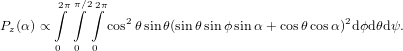
Abstract
The fluorescence anisotropy is calculated for a system in which the angle between absorption and emission dipole is not fixed but is given by a distribution around a central value and may have an additional degree of freedom in form of a rotation on an axis perpendicular to the excitation dipole. First, a so-called parallel transition is considered, where the two dipoles have the same direction. Then, the general expression for a fixed, non-zero angle is derived. Finally, an integration over a range of values yields the desired result. 1
The anisotropy to be expected from a molecule where excitation and emission (or probe-) dipole are not parallel can be calculated by the well-known formula
|
| (1) |
where α is the angle between the two dipoles. In a situation where these dipoles are localised on two different moieties of a molecule or complex which are not rigidly linked, this formula cannot be used any more. To extend it to such a scenario we’ll first derive the above formula and insert afterwards the additional degree of freedom at the appropriate step.
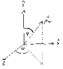
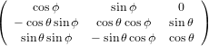
Let us first consider a molecule with a so-called parallel transition, i.e. an excitation-emission cycle in which the transition dipoles for excitation and emission are parallel to each other. These dipoles shall be characterised by their moduli μ21 and μ32 and the two angles ϕ and ψ, where ϕ describes the angle between the dipole and the z-axis, whereas ψ denotes the angle between the projection of the dipole onto the x-y plane and the x-axis (c.f. figure 1).
We chose the excitation source to be polarised parallel to the z-axis. The emission from
the dipole  32 is detected along the x-axis, using polarisations in two directions, parallel to
the z-axis and parallel to the y-axis, respectively. The probability of detecting a photon in
one of the two directions when exciting a molecule oriented in space according to ϕ and ψ
is proportional to the product of the probability of exciting the molecule, the probability
of detecting a photon emitted by an excited molecule and by the detection efficiency. The
constant of proportionality is determined by the absorption cross section and the quantum
efficiency of the photo cycle in the molecule, and by the solid angle of detection. The z- and
y-components of the electric field emitted by an excited molecule at angles ϕ and ψ are given
by
32 is detected along the x-axis, using polarisations in two directions, parallel to
the z-axis and parallel to the y-axis, respectively. The probability of detecting a photon in
one of the two directions when exciting a molecule oriented in space according to ϕ and ψ
is proportional to the product of the probability of exciting the molecule, the probability
of detecting a photon emitted by an excited molecule and by the detection efficiency. The
constant of proportionality is determined by the absorption cross section and the quantum
efficiency of the photo cycle in the molecule, and by the solid angle of detection. The z- and
y-components of the electric field emitted by an excited molecule at angles ϕ and ψ are given
by
| Ez(ϕ,ψ) | = Ez(ϕ) = E cosϕ | (2) |
| Ey(ϕ,ψ) | = E sinϕsinψ. | (3) |
| Pdet,z(ϕ) | ∝ Iz(ϕ) = E02 cos2ϕ | (4) |
| Pdet,y(ϕ,ψ) | ∝ Iy(ϕ,ψ) = E02 sin2ϕcos2ψ, | (5) |
 21 oriented according to ϕ and ψ is given
by
21 oriented according to ϕ and ψ is given
by
 | (6) |
The total probability to detect a photon coming from a single molecule and being polarised parallel to the z- or y-axis is therefore the product of the corresponding probabilities
| Pz(ϕ) | = Pex(ϕ)Pdet,z(ϕ) ∝ cos4ϕ | (7) |
| Py(ϕ,ψ) | = Pex(ϕ)Pdet,y(ϕ,ψ) ∝ cos2ϕsin2ϕcos2ψ. | (8) |
 | (9) |
The origin of the factor sinϕ can be explained as follows. Integrating dϕdψ over ψ from 0 to 2π at ϕ close to 90 ∘ yields a much larger value than at ϕ close to zero. The values of these integrals are represented by the corresponding part of the surface of a sphere. A stripe around the equator of with Δϕ will have a much larger surface than a one close to the pole of the same width. The ratio between the surfaces is given by sinϕ. We have therefore
| Pz | = ∫ 02π ∫ 0π∕2P z(ϕ)sinϕdϕdψ | (10) |
| ∝ 2π ∫ 0π∕2 cos4ϕsinϕdϕ | (11) | |
= −2π 0π∕2 0π∕2 | (12) | |
=  , , | (13) |
 | (14) |
The probability of detecting a photon polarised in y-direction is similarly given by
| Py | = ∫ 02π ∫ 0π∕2P y(ϕ,ψ)sinϕdϕdψ | (15) |
| ∝∫ 02π ∫ 0π∕2 cos2ϕsin2ϕcos2ψdϕdψ | (16) | |
= π ∫
0π∕2 cos2ϕ sinϕdϕ sinϕdϕ | (17) | |
= −π![[ ]
1cos3ϕ − 1cos5ϕ
3 5](anisotropy11x.png) 0π∕2 = 0π∕2 =  π. π. | (18) |
 | (19) |
since the constants of proportionality do not depend on the polarisation and are, therefore, the same for parallel and perpendicular detection.
We assume now that the two transition dipoles  21 and
  32 are separated by an angle α. The problem
becomes a little more complicated as we also have to take into account now the orientation of the plane
spanned by
32 are separated by an angle α. The problem
becomes a little more complicated as we also have to take into account now the orientation of the plane
spanned by  21 and
  32. In other words, given a certain orientation of
  21 as in the previous section and
fixing α, we may still rotate the molecule around
21 as in the previous section and
fixing α, we may still rotate the molecule around  21. Excitation source and emission detection are fixed
within the lab coordinate system {
21. Excitation source and emission detection are fixed
within the lab coordinate system { i} = {
 ,ŷ,ẑ} = {
 1,
1, 2,
2, 3}, whereas the orientation of the
transition dipoles is more easily described in a molecule-internal coordinate system {êi} = {ê1,ê2,ê3}.
The idea of the calculation is similar to the parallel transition, however, we first have to express the
molecule-internal coordinate system in terms of the laboratory coordinate system. In general, the
transformation of a rectangular and right handed coordinate system into another can be performed by
two rotations. However, as the two corresponding axes are in general not parallel to one of the
axes of the coordinate systems, a calculation using these two rotations is rather complicated.
Euler’s method simplifies the description at the cost of introducing an additional rotational
transformation.
3}, whereas the orientation of the
transition dipoles is more easily described in a molecule-internal coordinate system {êi} = {ê1,ê2,ê3}.
The idea of the calculation is similar to the parallel transition, however, we first have to express the
molecule-internal coordinate system in terms of the laboratory coordinate system. In general, the
transformation of a rectangular and right handed coordinate system into another can be performed by
two rotations. However, as the two corresponding axes are in general not parallel to one of the
axes of the coordinate systems, a calculation using these two rotations is rather complicated.
Euler’s method simplifies the description at the cost of introducing an additional rotational
transformation.
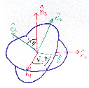
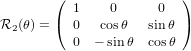
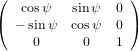
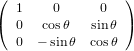
Figure 2 illustrates the threefold angular transformation. The two circles indicate the
planes spanned by  1 and
1 and  2, and by ê1 and ê2, respectively. In a first step, the laboratory
system {
2, and by ê1 and ê2, respectively. In a first step, the laboratory
system { i} is rotated around the
  3 axis by an angle ϕ such that the new vector
  1′ is
identical with the intersection line of the two circles. We have
1′ is
identical with the intersection line of the two circles. We have  3′ =
3′ =  3, and the
  1-
1- 2 circle is
conserved during this rotation. The second step consists of a rotation around the new vector
2 circle is
conserved during this rotation. The second step consists of a rotation around the new vector
 1′ by θ such that
  3′′ becomes equal to ê3. This rotation tilts also the
  1-
1- 2 plane into
the ê1-ê2 plane. Finally, the obtained system is turned around ê3 =
2 plane into
the ê1-ê2 plane. Finally, the obtained system is turned around ê3 =  3′′ by ψ such that
{
3′′ by ψ such that
{ i′′′}≡{êi}.
Mathematically, the first step is described by the three following equations
 1′ 1′ | = cosϕ 1 + sinϕ
 2 2 | (20) |
 2′ 2′ | = −sinϕ 1 + cosϕ
 2 2 | (21) |
 3′ 3′ | =  3
3 | (22) |
 | (23) |
with
 | (24) |
Similarly we have
 1′′ 1′′ | =  1′
1′ | (25) |
 2′′ 2′′ | = cosθ 2′ + sinθ
 3′
3′ | (26) |
 3′′ 3′′ | = −sinθ 2′ + cosθ
 3′
3′ | (27) |
 | (28) |
and
| ê1 | = cosψ 1′′ + sinψ 1′′ + sinψ 2′′
2′′ | (29) |
| ê2 | = −sinψ 1′′ + cosψ 1′′ + cosψ 2′′
2′′ | (30) |
| ê3 | =  3′′ 3′′ | (31) |
 | (32) |
Combining the rotations together we get
 | (33) |
The transformation matrix is given by the matrix multiplication of the three individual transformation matrices
 (ψ,θ,ϕ) = (ψ,θ,ϕ) = | (34) | ||
   | |||
=   | (35) | ||
= 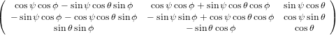 . . | (36) |
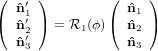
(ψ,θ,ϕ) we can now express {êi} by { i} as
i} as
 | (37) |
with
![dij(ψ,θ,ϕ) = [D(ψ,θ,ϕ)]ij.](anisotropy75x.png) | (38) |
Let us assume that  21 is parallel to ê3
 | (39) |
and that  32 lies in the plane spanned by ê1 and ê3
 | (40) |
where α denotes the angle between  21 and
  32. This choice has been made such that using Euler’s
transformation will not only yield an expression of the molecule’s orientation in the laboratory
coordinate system, but will also yield a direct parametrisation of the most important angles. θ represents
the angle between the z-axis (the direction of the polarisation of the excitation light) and
the excitation dipole μ21. ψ indicates the rotation of the molecule around μ21, the added
degree of freedom in the problem. And ϕ, finally, parametrises the rotation of μ21 around the
z-axis.
32. This choice has been made such that using Euler’s
transformation will not only yield an expression of the molecule’s orientation in the laboratory
coordinate system, but will also yield a direct parametrisation of the most important angles. θ represents
the angle between the z-axis (the direction of the polarisation of the excitation light) and
the excitation dipole μ21. ψ indicates the rotation of the molecule around μ21, the added
degree of freedom in the problem. And ϕ, finally, parametrises the rotation of μ21 around the
z-axis.
Expressed in the laboratory coordinate system the excitation dipole reads
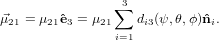 | (41) |
The emission dipole moment is given by
![∑3
⃗μ32 = μ32 [di1(ψ,θ,ϕ)sinα + di3(ψ,θ,ϕ)cosα]ˆni.
i=1](anisotropy83x.png) | (42) |
The intensity of the emitted light with polarisation in z-direction is again the square of the projection of
 32 onto ẑ, i.e. the square of the z-component of (42)
| Iz(ψ,θ,ϕ) | = E02[d 31(ψ,θ,ϕ)sinα + d33(ψ,θ,ϕ)cosα]2 | (43) |
| = E02(sinθ sinϕsinα + cosθ cosα)2 | (44) |
| Iy(ψ,θ,ϕ) | = E02[d 21(ψ,θ,ϕ)sinα + d23(ψ,θ,ϕ)cosα]2 | (45) |
| = E02[(−sinψ cosϕ − cosψ cosθ sinϕ)sinα + cosψ sinθ cosα]2. | (46) |
| Pz(ψ,θ,ϕ,α) | ∝ cos2θ(sinθ sinϕsinα + cosθ cosα)2 | (47) |
| Py(ψ,θ,ϕ,α) | ∝ cos2θ[(−sinψ cosϕ − cosψ cosθ sinϕ)sinα + cosψ sinθ cosα]2. | (48) |
 | (49) |
The integration over ψ yields a constant factor 2π, and due to the factor sinϕ, the cross term of the bracket vanishes when integrating over ϕ from 0 to 2π. We have therefore
 | (50) |
Using sin2θ = 1 − cos2θ we get
| Pz(α) | = 2π2 ∫
0π∕2 sinθ![[ ( ) ]
cos4θ 2 cos2α − sin2α + cos2θ sin2α](anisotropy87x.png) dθ dθ | (51) |
= −2π2![[ ]
1 (2cos2α− sin2α)cos5θ+ 1 sin2α cos3θ
5 3](anisotropy88x.png) 0π∕2 0π∕2 | (52) | |
=  π2 cos2α + π2 cos2α +  π2 sin2α π2 sin2α | (53) | |
=  π2 π2 . . | (54) |
![∫2ππ∫∕22∫π
Py(α) ∝ cos2θ sinθ [(− sinψ cosϕ− cosψ cosθsin ϕ)sinα + cosψ sinθcosα ]2dϕdθdψ.
0 0 0](anisotropy93x.png) | (55) |
The integration over ϕ is again easily performed, as ϕ occurs only in the first term of the square bracket. Therefore, the cross terms vanish when integrating over ϕ from 0 to 2π. We have thus
| Py(α) | = π ∫
02π ∫
0π∕2 cos2θsinθ | (56) | |
+ ![]
2cos2 ψsin2 θcos2 α](anisotropy95x.png) dθdψ dθdψ | |||
= π2 ∫
0π∕2 cos2θsinθ dθ dθ | (57) | ||
= π2![[ ]
− 1 sin2α cos3θ− 1 sin2α cos5θ − 2cos2α cos3θ + 2cos2α cos5θ
3 5 3 5](anisotropy97x.png) 0π∕2 0π∕2 | (58) | ||
=  π2 π2 . . | (59) |
 | (60) |
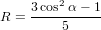
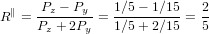
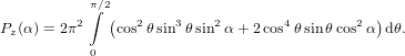
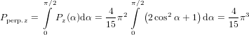
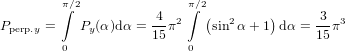
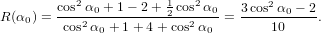
For α = 0∘ we get again R∥ = 0.4 as already found in (19) in the previous section. For a perpendicular
transition, i.e. α = 90∘, we get R⊥ = −0.2. For a complete arbitrary orientation of the two
dipoles—which should yield an isotropic signal—we have to integrate over α, taking into account that
varying α is possible by turning  32 in two independent directions within the molecule-internal
coordinate system. This is reflected in an additional factor sinα (c.f. (9) and the subsequent
phrase)
32 in two independent directions within the molecule-internal
coordinate system. This is reflected in an additional factor sinα (c.f. (9) and the subsequent
phrase)
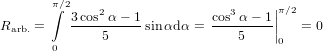 | (61) |
as expected.
In some molecules the emission can occur from two degenerated states with transition dipoles perpendicular to each other. (60) can be used directly with α = 90∘ when the plane spanned by these two dipoles is perpendicular to the transition dipole which corresponds to the excitation. The integration over ψ in the above derivation, being there an average over all molecules in the sample, can also be interpreted as the integration over all possible emission directions within the same molecule. We get R = −0.2 in this case.
On the other hand, an integration over α from 0∘ to 90∘ will yield the anisotropy for the case where the plane spanned by the two emission dipoles contains the excitation dipole. However, performing the calculation of Pz and Py we do not need to care about normalisation due to averaging over solid angles as the normalisation is the same for both polarisations and will thus vanish when calculating R.
 | (62) |
and
 | (63) |
We have thus
 | (64) |
A distribution of directions wα can be introduced using (60)
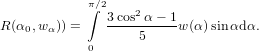 | (65) |
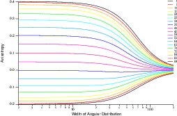
Figure 3 shows the anisotropy R of a distribution of angles around α for a couple of equidistant angles between zero an 90 ∘. Note the logarithmic scale for the width of the Gaussian distribution.
Let us assume that the probed dipole is not rigidly attached to the excitation dipole but may freely
rotate around an axis perpendicular to the excitation dipole. This situation could correspond to a weakly
bound complex of two planar molecules in a sandwich-like geometry where the mutual orientation is
random with respect to the normal direction of the “sandwich plane”. Let us start from the geometry
where the angle between the dipoles is minimal and let us call this minimal angle α0. Turning the probe
dipole around the vector which is perpendicular to  12 and lies in the plane spawned by
  12 and
 23(0) generates the set of contributing molecules, where
  23(0) is the probe dipole which
corresponds to the minimal angle α0. An integration over the turning angle δ yields the desired
result. However, as (60) is not linear neither in Py(α) nor in Pz(α), we have to perform the
integration in these two expressions using (51) and (56) and to calculate R(α0) by the usual
expression.
23(0) is the probe dipole which
corresponds to the minimal angle α0. An integration over the turning angle δ yields the desired
result. However, as (60) is not linear neither in Py(α) nor in Pz(α), we have to perform the
integration in these two expressions using (51) and (56) and to calculate R(α0) by the usual
expression.
From fig. 1 and using (40) we obtain
 | (66) |
The relation between α and γ is given by the scalar product
 | (67) |
where we have used again (40). For the detection probability with polarisation parallel to the z-axis we obtain therefore using (51)
| Pz(α0) | = ∫ 0π∕2P z(α(γ,α0))dγ | (68) |
=  π2 ∫
0π∕2 π2 ∫
0π∕2![{ 2 }
2cos [arccos(cosα0 cosγ )]+ 1](anisotropy115x.png) dγ dγ | (69) | |
=  π2 ∫
0π∕2 π2 ∫
0π∕2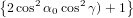 dγ dγ | (70) | |
=  π3 π3 . . | (71) |
 | (72) |
we get similarly for detection with polarisation parallel to the y-axis
| Py(α0) | = ∫
0π∕2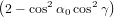 dγ dγ | (73) |
=  π3 π3 . . | (74) |
 | (75) |
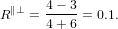
Considering the two extreme cases α0 = 0 and α0 = π∕2 yields the known values of R = 0.1 and R = −0.2, respectively, as to be expected. In between, no new maximum is to be observed. In other words, in the situation described here, the maximum positive anisotropy to be obtained is R = 0.1.
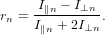
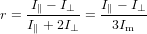
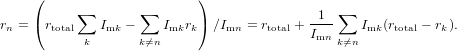
Assume that the detected signal is composed out of several different contributions which are of different absolute intensity and anisotropy. The anisotropy rn for the nth contribution as an isolated signal is given by the usual definition
 | (76) |
It is important to notice that the total anisotropy is not the sum or average of the individual anisotropies but the anisotropy of the sum of the signals
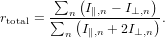 | (77) |
In consequence, the total anisotropy is a nonlinear quantity with respect to the individual contributions. Let us inspect how this total anisotropy looks like. We start from the usual definition of the anisotropy
 | (78) |
with Im being the signal at magic angle
 | (79) |
or equivalently
 | (80) |
and
 | (81) |
Inserting (80), respectively (81) into (78) we have
 | (82) |
and
 | (83) |
as can easily be verified by inserting (82) and (83) into (78). Inserting (82) and (83) into (77) we get
![-∑n-Imn[(2rn-+1)-− (1-− rn)] ∑n-Imnrn-
rtotal = ∑ Imn [(2rn + 1)+ 2(1− rn)] = ∑ Imn .
n n](anisotropy133x.png) | (84) |
The obtained formula resembles the one which determines the position of the center of masses in an ensemble of particles. Hence, for positive magic angle signals Im the total anisotropy lies always in between the anisotropy values of the individual contributions and closest to the anisotropy value of the contribution with the largest absolute signal at magic angle.
Special attention has to be payed in case of contributions which may have opposite signs as for instance data obtained from a transient absorption measurement in spectral regions with overlap of induced absorption and emission or bleach signals. When two contributions with opposite sign cancel each other, i.e. the corresponding magic angle signal crosses the zero line, the denominator of (84) vanishes and rtotal diverges. In the vicinity of such a zero-crossing point any value between −∞ and +∞ can be obtained for rtotal depending on the detailed experimental conditions like signal-to-noise ratio and removal of background offset signals. But even without a zero-crossing nearly arbitrary values may be obtained for rtotal in case of two contributions with large anisotropy of the same sign but signal of opposite sign and similar amplitude. As soon as ∑ nImn ≪∑ n|Imn| one has to be prepared for “surprises”. In consequence, when trying to extract from the measured anisotropy the anisotropy of an individual contribution to the signal can be difficult. It is given by the expression
 | (85) |
If all but one anisotropy values rk,r≠n and all intensities Imk have been determined, the missing rn can be calculated. To estimate the uncertainty in rn we need to calculate the derivations with respect to all parameters
 | = 1 + (Itotal − Imn)∕Imn = Itotal∕Imn | (86) |
 | = (rtotal − rk)∕Imn | (87) |
 | = −Imk∕Imn | (88) |
 | = − ∑
k≠nImk(rtotal − rk). ∑
k≠nImk(rtotal − rk). | (89) |
Another word of caution should be added. Also when dealing with composed signals, in general the total anisotropy of a sample decays eventually to zero, respectively to some residual value. Depending on the underlying kinetics the decay may or may not be monotonic. When the decay is monotonic, it might be tempting to describe the obtained curve by an exponential function or a sum of such. However, if the underlying contributions do not share the same kinetics, the obtained exponential terms will have nothing to do with the signals or anisotropies of the individual components because the dependence of the total anisotropy on the individual anisotropies of the different contributions is nonlinear. A proper decomposition has always to refer to (84).