Deconvolving Auto- and Crosscorrelation Traces
When extracting the pulse width from an autocorrelation curve, two points have to be taken into
account:
- the relation between the value obtained for the corresponding fit parameter and the
full-width-half-maximum (FWHM) of the curve,
- and the relation between the width of a curve and the width of the curve obtained
by convoluting the curve with itself.
1 Gaussian width and FWHM
When fitting a Gaussian curve, the model function is usually
 | (1) |
where τ is the parameter controlling the width. The relationship to the FWHM is given by the
condition
The FWHM ΔT is then given by
 | (5) |
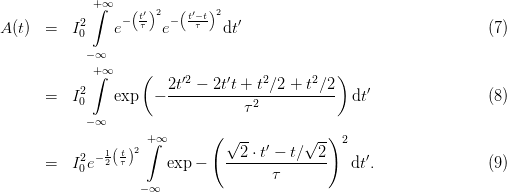
2 Convolving a Gaussian with itself
Assuming a laser pulse with a Gaussian envelope
 | (6) |
the autocorrelation curve can be described as
Since this integral is infinite, a constant offset in the integration variable does not change the
value of the integral. Thus, the integral does not depend on t. In consequence, the obtained
function is again a Gaussian curve (time dependent term before the integral) and a constant
factor, given by the value of the infinite integral
 | (10) |
The width of this Gaussian curve is thus  times larger than the original curve.
Therefore, the laser field expressed by the FWHM ΔT reads
 | (11) |
When fitting a Gaussian to an autocorrelation curve, the relation between fit parameter τ as
given in (1) and FWHM ΔT of the pulse is
 | (12) |
3 Third Order Autocorrelation
In a third order autocorrelation one of the fields enters twice into the expression and the
measured signal becomes
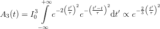 | (13) |
where the integral has been evaluated as before. As FWHM ΔT3 for the deconvoluted pulse
width we get therefore
 | (14) |
4 Cross Correlation
A cross correlation of two pulses with Gaussian profile of duration τ1 and τ2, respectively, is
described by a convolution of the two Gaussians
The result is a Gaussian with a width given by the geometrical mean of the widths
of the two convoluted pulses. Its amplitude is strictly monotonously increasing with
decreasing pulse duration of either pulse when keeping the other one fixed. In case of
τ1 ≫ τ2 the width is equal to τ1 and the peak intensity scales with 1∕τ1, and vice
versa.
![+∫∞ (t′)2 (t′−t)2
C (t) = I0,1I0,2 e− τ1 e− -τ2- dt′ (15)
τ1τ2π
−∞
+∫∞ [ 2 2 ′2 2′ 22 ]
= I0,1I0,2 exp − (τ2-+-τ1)t--−-2τ1-tt +-τ1-t dt′ (16)
τ1τ2π τ12τ22
−∞ [ ]
I0,1I0,2 τ12t2-−-τ41t2∕(τ21 +-τ22)
= τ τ π exp − τ 2τ 2
1 2 ⌊ ( ∘ -1-2---- ∘ -------)2⌋
+∫ ∞ t′ τ 2+ τ2 − τ2t∕ τ2+ τ 2
× exp |⌈− ------1----2----1------1---2---|⌉ dt′ (17)
τ12τ22
− ∞
[ ] +∫ ∞ ( ∘ --------)2
I0,1I0,2 21-−-τ21∕(τ21-+-τ22) ′--τ12+-τ22- ′
= τ1τ2π exp − t τ2 exp − t τ1τ2 dt (18)
2 − ∞
I0,1I0,2 ( t2 )
= ∘------------exp − -2----2- . (19)
π(τ21 + τ22) τ1 + τ2](autocorrelation11x.png)