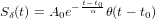
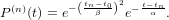
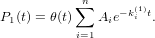
The temporal evolution of the population of a state excited by a delta-like perturbative action at time t0 can be described as
|
| (1) |
for all positive and negative times, where θ(t) denotes the heavyside step function
 | (2) |
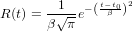
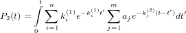
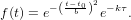
In a real experiment excitation and detection have a finite duration, setting up together the experiment response function which we assume here to be of Gaussian shape
 | (3) |
where the area under the infinite integral has been normalised to unity
 | (4) |
as to preserve the absolute signal intensities. For the moment we focus on the excitation time-profile and put aside the detector response time which is to be treated later.

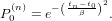
Figure 1 shows a sketch of the times involved. For a delta-like excitation at time tn the contribution to the excited state population corresponds to the value of the excitation profile at tn
 | (5) |
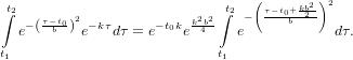
The population of this “excitation-slice” which is left at time t is given by the decay since the excitation at tn. At time t, excitation at time tn contributes therefore with
 | (6) |
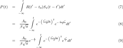
Here we have to keep tn ≤ t since the negative part of the exponential function on the left side would lead to an unphysical situation. The overall signal at time t is therefore given by the sum over all “excitation-slices” ∑ nP(n)(t), which turns into the convolution of the the two functions R and Sδ once we let the size of the “excitation-slices” go to zero. The upper limit guarantees t′ ≤ t.
This integral can be solved using (47) with b = β and k = −1∕τ and we get
![[ ( β2) ]
P(t) = A0-e− t−τt0e4β2τ2 1 +erf t−-t0 −-2τ
2 β](convoluted-exponential7x.png) | (10) |
where erf() denotes the error function (cf. eqn. 42). An extension to a multi-exponential decay is straight forward and leads to a sum of exponentials and therefore to a sum of convolutions like the one shown here.
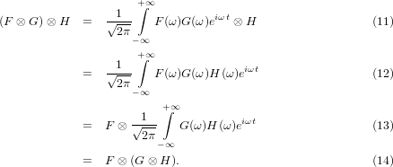
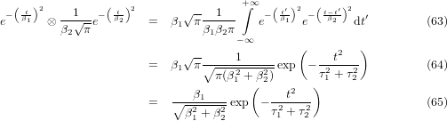
The detection of this population involves a second convolution with a Gaussian function of width β2. The convolution theorem tells us that a twofold convolution with a Gausssian is nothing but a convolution with the two convoluted Gaussians
 | (15) |
Imagine now a state being populated by a delta-exciation and decaying subsequently with a given rate constant into a second state. The observable shall be the population of the second state. The population of the first state is described as
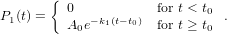 | (16) |
The time dependent arrival of the population in the second state is then given by the derivative of the population of the first state multiplied by minus one. If the second state does not decay (or only very slowly), the population is accumulated as
![t
∫ dP1(τ) [ − k1(t− t0)]
P2(t) = − --dτ--dτ = P1(t0)− P1(t) = A0 1 − e .
t0](convoluted-exponential11x.png) | (17) |
When the second state already decays during the arrival of new population, the transient population P2 is given by a convolution
![∫t [ ]
dP1(τ) − k2(t− τ)
P2(t) = − dτ e dτ (18)
t0
∫t
= A0k1 e−k1(τ−t0)e−k2(t−τ)dτ (19)
t0
∫t
−k2t+k1t0 − (k1−k2)τ
= A0ke e dτ. (20)
t0](convoluted-exponential12x.png)
 | (21) |
For k1≠k2 the integral has to be evaluated and we get
For k1 > k2, i.e. the transition from state 1 to state 2 being faster than the emptying of state 2, this function exhibits an exponential rise with rate k1 and a subsequent decay with rate r2 as expected. For k1 ≫ k2 the small contribution of k2 in the denominator can be neglected and we get
![P (t) ≈ A [e−k2(t−t0) − e−k1(t− t0)].
2 0](convoluted-exponential15x.png) | (24) |
However, for k1 < k2, i.e. when state 2 is emptied faster than it is populated, the sign of the pre-factor changes, which is the same as interchanging the two terms in the bracket. Thus, again we get a rise and a subsequent decay, but now the raise corresponds to the emptying (k2) and the decay corresponds to the arrival (k1). It is just the mathematics of a convolution of two exponential functions which yields that the step with the higher rate constant will appear as rise. The slower one always appears as decay. For k1 ≪ k2 the contribution of k2 in the denomiator is small and can be neglected. We get thus
![[ ]
P2(t) ≈ A0k1 e− k1(t−t0) − e−k2(t−t0) .
k2](convoluted-exponential16x.png) | (25) |
The interchange of rise and decay is clearly to be seen, as well as a lowering of the maximum by the ratio of the time constants k1∕k2.
Multiple exponential decays of both states can be treated in the same way as the convolution is a linear operation in both involved functions. Let now P1(t) be defined as
 | (26) |
The decay of P2 should be also given by a multi exponential function. We have then
 | (27) |
with the condition
 | (28) |
This leads obviously to n × m terms, each of them being the convolution of two mono-exponential functions. According to (23) we get
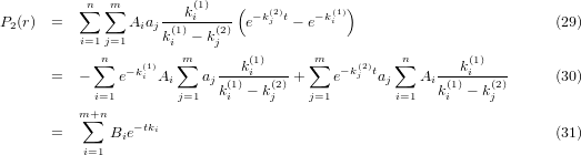
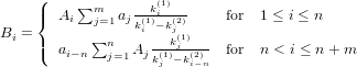 | (32) |
In the following some often used integrals are given.
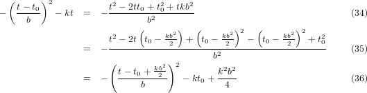
Any product of a Gaussian function and an exponential decay can be described by
 | (33) |
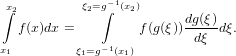
For an integration of this expression it is much more simple to rewrite the exponent as
Therefore, the integral of the product can be written as
 | (37) |
By the substitution
 | (38) |
and using the chain rule for integrals
 | (39) |
we may write
 | (40) |
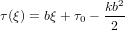
with
 | (41) |
The integral equals now to the definition of the error function
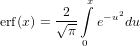 | (42) |
being the positive half of the integral of a Gaussian function.

Using the definition of the error-function for negative values
 | (43) |
the symmetry of the Gaussian function
 | (44) |
and its infinite integral
 | (45) |
one can easily show that
![x∫2 √ --
e−u2du =--π[1+ erf(x)]xx21.
x1 2](convoluted-exponential33x.png) | (46) |
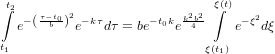
Figure 2 illustrates these properties of the error-function. We have thus
![∫t2 τ−t 2 √ -- 22[ ( kb2)]
e−(-b0) e−kτdτ = b-πe− t0kekb4- 1 + erf t−-t0 +-2-
t1 2 b](convoluted-exponential34x.png) | (47) |
Any product of the integral of the Gaussian function and an exponential decay can be described by
![[ (τ − τ )]
f (τ) = e−kτ 1+ erf -----0 .
b](convoluted-exponential35x.png) | (48) |
Using the product rule of differentiation
 | (49) |
We chose
![u′(τ) = e−kτ (50)
[ (τ − τ0)]
v(τ) = 1+ erf --b--- (51)](convoluted-exponential37x.png)
![∫t2 [ ( ) ]
−kτ τ −-τ0
F(t) = e 1 + erf b dτ (54)
t1
1 [ ( τ − τ )]t2 1 t∫2 τ−τ 2
= − -e−kτ 1 +erf ----0- + -- e−kτe−(-b0) dτ (55)
k b t1 kb t1
( √-- [ ( 2)]t2)
= 1-{[f(t) − f (t )]+-π-ek2b42e−τ0k 1+ erf τ −-τ0 +-kb2 } . (56)
k ( 1 2 2k b )
t1](convoluted-exponential39x.png)
![+∫∞ ( ) ( )
--1--- − tβ′1 2 − t−βt2′ 2 ′
β1β2π e e dt (58)
− ∞
1 +∫∞ ( (β2 + β2)t′2 − 2β2tt′ + β2t2)
= ------ exp − -2----1---2-2-1-----1-- dt′ (59)
β1β2π −∞ β1β2
( ∘------- β2t ) 2
1 [ β2t2 − β4t2∕(β2 + β2)] +∫ ∞ | β21 + β22t′ − √β121+β22|
= β-βπ-exp − -1-----1β2β2-1----2- exp( − -------β-β--------) dt′ (60)
1 2 1 2 −∞ 1 2
[ ] +∫∞ ( ∘ -------)2
--1--- 21−-β21∕(β21 +-β22) ′--β21 +-β22 ′
= β1β2π exp − t β22 exp − t β1β2 dt (61)
( ) −∞
= ∘----1-----exp −---t2--- . (62)
π(β21 + β22) τ21 + τ22](convoluted-exponential41x.png)
![---k1-- k1t0− k2t[ −(k1− k2)τ]t
P2(t) = A0k1 − k2e e e t0 (22)
k1 [ ]
= A0k--−-k- e−k2(t−t0) − e−k1(t−t0). (23)
1 2](convoluted-exponential14x.png)
![∫t [ ( )] { [ ( ) ]
e−kτ 1+ erf τ −-τ0 dτ = 1- − e−kt 1+ erf t−-τ0 (57)
b k b
− ∞ √ -- [ ( 2)] }
--π −τ0k k2b42 t−-τ0 +-kb2
+ 2 e e 1 + erf b .](convoluted-exponential40x.png)