Abstract
This document sums up a collection of properties of the Fourier transformation. Attention is payed to keep all scalings and norms correct so that the formulas can be used for quantitative calculations.
The origin of the Fourier transformation is connected to the research on string vibrations and heat conductivity around 1800. The famous book La Théorie Analytique de la Chaleur, published in 1822 by Joseph Fourier, gave the mathematical tool of frequency analysis its name. While the acoustical application–decomposing a sound into its harmonics–sounds somewhat generic in our days, the connection between trigonometric functions, frequency analysis and heat conductivity isn’t obvious. Let us shortly demonstrate it.
Suppose that we have an infinite slab of a uniform conducting material of thickness d and an initial temperature distribution T0(x). The temperature outside this medium should be zero. We are asking for the temperature distribution T(t,x). The physical theory tells us that heat conduction is governed by the differential equation
|
| (1) |
where k is a constant describing the conductivity of the material. We have the boundary conditions
 | (2) |
Making a separation ansatz T(x,t) = g(x)h(t) we get
 | (3) |
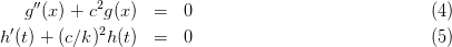
Since each side of this equation contains only one variable, both sides must be equal to the same constant which we may call −c2. Thus we get two separate differential equations
which are easily solved by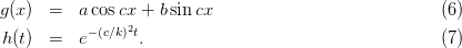
 | (8) |
The boundary condition T(0,t) = 0 can only be fulfilled by a = 0. Since b cannot also be zero, the boundary condition T(d,t) = 0 tells us that we have to have sin dc = 0 and hence cd must be a multiple of π, say c = nπ∕d. Thus, each value of n gives a solution
 | (9) |
Obviously, the boundary condition T(x, 0) = T0(x) cannot be fulfilled in general by just one of these solutions. But (omitting questions of convergence) we may construct an appropriate sum of these solutions which fulfilles the condition, as
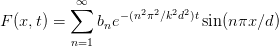 | (10) |
The boundary condition demands
 | (11) |
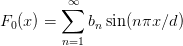
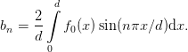
The remaining question is how to determine the coefficients bn. Without proof we use the relation
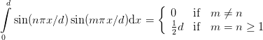 | (12) |
and get by multiplying with sin(mπx∕d) and integrating over the interval [0,d]
 | (13) |
If the initial temperature profile is constant T0(x) ≡ T we may easily calculate the full solution
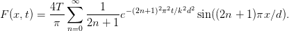 | (14) |
The development of a theory of heat conductivity thus lead to the discovery of trigonometric series. Another way to these series is the analysis of a string’s vibration which yields to a symmetric pair of equations similar to (4), one in t and one in x. The argument of the trigonometric functions in the equation of the time variable contains an angular frequency ω0 which is the lowest eigenfrequency of the string. The series is composed of trigonometrics in the harmonics (integer multiples) of this frequency
![∑∞
f (x,t) = g(x) [an cos(n ω0t) + bnsin (nω0t)].
n=1](fourier12x.png) | (15) |
All functions described by a series of this type are periodic with a periodicity of T = 2π∕ω0.
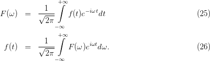
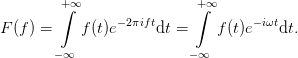
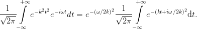
The way from a discrete trigonometric series towards a continuous Fourier integral is straight forward. As allways disregarding questions of convergence, we may send the periodicity to infinity T →∞ or ω0 → 0. The spacing of the harmonics gets narrower as we approach zero frequency and the sum converges to an integral when the limit is performed. This leads to the mathematical definition of the Fourier integral
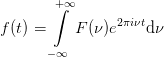 | (16) |
where the now continuous set of Fourier coefficients F(ν) is given by
 | (17) |
By substitution it can be shown that these two operations are invers to each other in the sense that performing the second on the result of the first or vice versa leaves the original function unchanged.
In the literature we find slightly different ways of defining the Fourier transformation. These differences concern the normalisation factors in forward and backward transformation and become important once a quantitative calculation is to be done. The mathematical definition implies more a direct link between time and frequency t ↔ ν than between time and angular frequency. The exponent 2πift = iωt involves the angular frequency ω = 2πf
 | (22) |
Substituting f by ω yields the often used time to angular frequency form
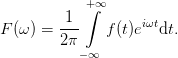 | (23) |
The need to keep normalisation tells us that the back transformation has in this case to be defined as
 | (24) |
as we can easily see by substitution in the upper calculation of one “roundtrip”. Yet another definition tries to get back the symmetry of the two formulas by distributing the normalisation factor equally over the two processes
Although being a trivial fact, it is important to note that F(ω) changes by a constant factor when changing from one of these definition to another.
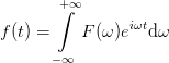
The convolution of two functions f(t) and g(t) is defined as
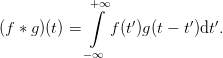 | (27) |
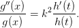
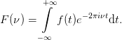
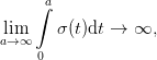
The convolution theorem states that the Fourier transform of a convolution is the direct product of the Fourier transforms
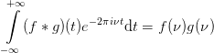 | (28) |
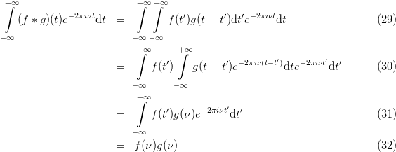
where we used the “mathematical” definition. The prove is easy
![+∫∞
FT [(f ∗ g )(t)] = -1- (f ∗ g)(t)e− iωtdt (33)
2π
−∞
+∫∞ +∫∞
= -1- f(t′)g (t − t′)dt′e−iωtdt (34)
2π
−∞ −∞
∫+∞ ∫+∞
= f (t′)-1- g (t − t′)e− iω(t− t′)dte −iωt′dt′ (35)
2π
−∞ −∞
∫+∞
= f (t′)g(ω)e−iωt′dt′ (36)
−∞
= 2πf (ω)g(ω ). (37)](fourier23x.png)
![+∫ ∞
--1-- −iωt √ ---
FT [(f ∗ g)(t)] = √ --- (f ∗ g)(t)e dt = 2π ⋅ f (ω)g(ω ).
2π− ∞](fourier24x.png) | (38) |
The Fourier transform of a Gaussian function with width τ has the width 2∕τ and a Gaussian with inverse width k has the width 1∕2k
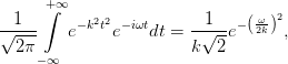 | (39) |
respectively
 | (40) |
This can be seen by completion of the square. The exponent in (39) reads
 | (41) |
We have thus
 | (42) |
The integral in this expression is an infinite integral over a Gaussian function on a straight line in
the complex plain which is parallel to the real axis. It can be solved by so-called compex contour
integration and yields a factor  ∕k, which proves (39).
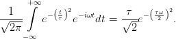
Suppose a function in time domain f(t) and its fourier transform f(ω). A time shift by some fixed amount t0 leads to a phase factor in frequency space
 = √-1-- f(t − t0)e−iωtdt (43)
2π
− ∞
+∫ ∞
= √-1-- f(t)e−iω(t+t0)dt (44)
2π
− ∞
+∫∞
= e−iωt0√-1-- f(t)e− iωtdt (45)
2π
−∞
= f(ω)e− iωt0. (46)](fourier30x.png)
The Fourier transformation obeys a general relationship for any complex-valued function f(x) and its Fourier transform f(ω). The Fourier transformation of the complex conjugate
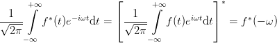 | (47) |
is the time-inverse of the complex conjugate of the Fourier transform. In other words, taking the complex conjugate inverses the direction of time in the Fourier transformation, respectively inverting time induces a complex conjugation in the Fourier transformation.
An immediate consequence of (47) is that for any real-valued function f(t) we have
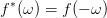 | (48) |
since for real-valued functions we have f(t) ≡ f∗(t). The positive half axis contains all information. The negative half axis is its complex conjugate.
Even and odd functions, f(−x) = f(x) and f(−x) = −f(x), respectively, play an important role in the transformations of symmetry in Fourier transformations. Any real- or complex-valued function f(x) can be written as the sum of an even and an odd function
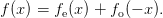 | (49) |
where fe(x) and fo(−x) can be constructed according to the following recipe
 | (50) |
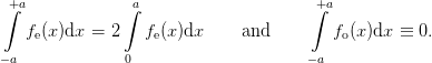
The following properties govern the transformation of symmetries. i) The product of two even functions as well as the product of two odd functions is even. ii) The product of an even and an odd functions is odd. iii) The sum of two even functions is even and the sum of two odd function is odd. iv) The sum of an even and an odd function is neither even nor odd. v) Integrating an even function symmetrically around zero yields obviously two times the integral over the part on the posive half axis. Likewise the same integral over an odd function vanishes.
 | (51) |
Using Euler’s rule we can split the exponential term in the Fourier transformation in its real and imaginary part with the real part being even and the imaginary part being odd.
![+∫∞ +∫∞
√1--- f(t)e−iωtdt = √1--- f(t)[cos(ωt) − isin(ωt )]dt.
2 π 2π
−∞ −∞](fourier36x.png) | (52) |
If f(t) is even, the part of the integral containing the sin function will vanish. We can therefore state that for even functions, a Fourier transformation is actually a cosine transformation. The real part of the Fourier transform stems entirely from the real part of f and the imaginary part entirely from the imaginary its part, respectively. For odd functions, the Fourier transformation reduces to a sine transformation where the real part of the Fourier transformation stems form the imaginary part of f and vice versa. These both conditions follow also from the fact that the mixed sum of even and odd functions is neither even nore odd. Together with the fact that the different terms of a Fourier series never cancel each other out to zero on the entire axis we can state that even functions can only displayed using a series of even functions and odd functions only using odd functions, respectively.
Furthermore, the Fourier transformation of a real-valued and even function is purely real. And due to (48) it is even too. Likewise, the Fourier transformation of a real-valued and odd function is purely imaginary and odd.
The Kramers-Kronig relation states that due to causality, real and imaginary part of the Fourier transformation of a response function depend on each other in a distinct way. The way the the mathematical representation of this relationship is presented in text books is often rather obscure due to the use of complex contour integrations. With the help of the “toolbox” set up in the previous sections we are able to limit this “obscurity” to the technical part where it belongs, the Fourier transformation of a step function.
The most general relation of a linear response X(t) of some physcial system to an applied external force f(t) can be described by a convolution
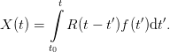 | (53) |
where R(t) is the linear response function of the system. Due to causality, R(t) must vanish for t < 0. Otherwise the system would exhibit a response before the cause having been applied. The equivalent formulation in freuquency domain is
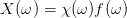 | (54) |
with
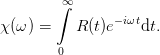 | (55) |
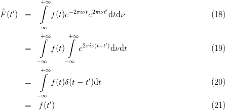
The lower integration limit is zero as R(t) vanishes on the negative half axis. We may now express R(t) as a sum of an even and an odd function. Instead of using (50) we use the obvious and equivalent way
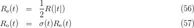
 | (58) |
Obviously, Re(t) + Ro(t) equals R(t) on the positive half axis and vanishes for t < 0. Applying the properties stated in the previous section we see that the Fourier transformation of the even part yields two times of (54). Furthermore, R(|t|) being even, its cosine transformation constitutes the real part of χ(ω)
![∫∞ ∫∞
1- −iωt
Re [χ(ω)] = 2 R (|t|)e dt = R (t) cos(ωt)dt.
− ∞ 0](fourier42x.png) | (59) |
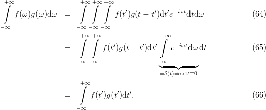
The odd part is a product of two functions. The corresponding Fourier transformation is therefore the convolution of the Fourier transformations of these functions
![∫∞
1- −iωt
Im [χ(ω )] = 2 σ (t)R (|t|)e dt = {FT [σ ] ⊗ Re (χ)}(ω ).
−∞](fourier43x.png) | (60) |
The calculation of Re(ω) we have already performed. It remains to compute the Fourier transformation of σ(t). This is, where the technical trick of a complex contour integration comes into play.
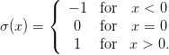
Without going through the details we may guess the important properties of the wanted function. i) As σ(t) contains a discontinuity at t = 0, its Fourier transformation must extend to infinity on both sides. ii) As σ(t) is entirely flat elsewhere, its Fourier transformation must have its most important contribution around zero frequency. iii) Since the infinite integral over σ(t) diverges
 | (61) |
the integral of its Fourier transformation must diverge too
dω → ∞.
a→0
a>0](fourier45x.png) | (62) |
iv) Furthermore, FT![[σ ]](fourier46x.png) (ω) must be odd. It happens that f(ω) = 1∕ω fulfilles all these
conditions. A complex contour integration shows, that i∕ω this indeed the Fourier transformation
of the sign function. Inserting this into (60) we obtain
(ω) must be odd. It happens that f(ω) = 1∕ω fulfilles all these
conditions. A complex contour integration shows, that i∕ω this indeed the Fourier transformation
of the sign function. Inserting this into (60) we obtain
![+∫∞
Re [χ(ω′)] ′
Im [χ (ω )] = − --ω-−-ω′--dω
−∞](fourier47x.png) | (63) |
which displays the Kramers-Kronig relation between the real and imaginary part of the susceptibility χ(ω).
Numerical computation of a Fourier transformation is in general performed using the so-called Fast-Fourier-Transformation or FFT algorithm based on the work of Cooley and Tukey [1]. It is interesting to note that this publication only made the method of efficient numerical calculations of Fourier transforms known to a broader public. In retrospective the algorithm had been found independently by more than a dozen individuals, starting with Carl Friedrich Gauss in 1805!